Bayesian Inference

Bayesian inference fully calculates the posterior probability distribution. Hence the output is not a single value but a probability density function(PDF) (when $\theta$ is a continuous variable) or a probability mass function(PMF) (when $\theta$ is a discrete variable)

Point estimator 인 Maximum Likelihood Estimation(MLE) 이나 maximum a posteriori probability(MAP) 와는 다르다.

• Bayesian inference 는 주로 point estimation 이 잘 먹히지 않을 때 사용한다.

2. 예시) 카지노 머신

두 카지노 기계 A, B 중 하나는 높은 확률 (67%) 로 상금을 준다.

두 기계를 돌려봤을때 전적은 다음과 같다.

• Machine A: 3 wins out of 4 plays
• Machine B: 81 wins out of 121 plays

MAP 를 통해 각 기계에 대한 parameter $\theta$ 를 구해보자.
만약, 기계 확률이 binomial distribution 을 따르고, prior 로 beta distribution 을 사용한다면, ${\hat{\theta }}_{MAP}=\frac{k+\alpha -1}{n+\alpha +\beta -2}$ 로 계산할 수 있다.

그럼 각 기계의 $\theta$ 는 다음과 같다.

• Machine A: (3+2–1)/(4+2+2–2) = 4/6 = 66.7%
• Machine B: (81+2–1)/(121+2+2–2) = 82/123 = 66.7%
  둘 다 동일한 $\theta$ 를 얻었기 때문에 어느 한쪽이 좋은 기계인지 알지 못한다.

반대로 Bayesian Inference 를 통해서 계산한 posterior probability 분포 $P(\theta \mid D)$ 는 다음과 같다.

$$P(\theta \mid D)=\frac{\Gamma (n+\alpha +\beta )}{\Gamma (k+\alpha )\Gamma (n-k+\beta )}{\theta }^{k+\alpha -1}(1-\theta {)}^{n-k+\beta -1}$$

위 식을 이용하여 각 기계 A, B 의 분포는 다음과 같이 그려진다.

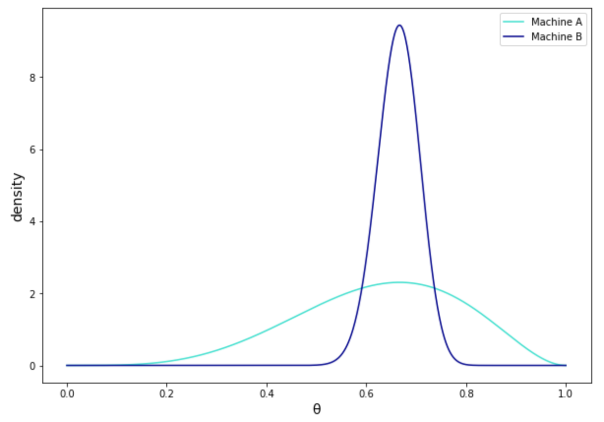
$\theta =\mathrm{0.6666..}$ 에서 각 분포가 mode 를 지니지만, 기계 A 가 B 보다 더 가파른 distribution 을 지닌다.

[MAP](maximum a posteriori probability) 와 Bayesian Inference 의 차이점은 Bayes theorem 에서 evidence $P(D)$ 를 계산하는 것에 있다.

• evidence 또는 marginal likelihood 라고도 한다.
• $\theta$ 가 continuous variable 인 경우, $\theta$ 는 joint probability 에 의해 계산한다.

$$P(D)={\int }_{\theta }P(D,\theta )d\theta ={\int }_{\theta }P(D\mid \theta )P(\theta )d\theta$$

두번째 식은 chain rule (probability) 에 의해 유도된다.

즉, Bayes theorem 은

$$P(\theta \mid D)=\frac{P(D\mid \theta )P(\theta )}{P(D)}=\frac{P(D\mid \theta )P(\theta )}{{\int }_{\theta }P(D\mid \theta )P(\theta )d\theta }$$

가 된다.

3. 예시

Binomial Distribution 을 따르는 likelihood 와 beta distribution 을 따르는 prior 의 경우

$$\begin{array}{l}P(D)={\int }_{\theta }P(D\mid \theta )P(\theta )d\theta \\ \\ ={\int }_0^1\left(\begin{array}{l}n\\ k\end{array}\right){\theta }^k(1-\theta {)}^{n-k}\frac{\Gamma (\alpha +\beta )}{\Gamma (\alpha )\Gamma (\beta )}{\theta }^{\alpha -1}(1-\theta {)}^{\beta -1}d\theta \\ \\ =\left(\begin{array}{l}n\\ k\end{array}\right)\frac{\Gamma (\alpha +\beta )}{\Gamma (\alpha )\Gamma (\beta )}{\int }_0^1{\theta }^{k+\alpha -1}(1-\theta {)}^{n-k+\beta -1}d\theta \end{array}$$

여기서 $\theta$ 는 Binomial Distribution 특성 상 확률을 의미하므로, 0 부터 1 사이의 값을 가질 수 밖에 없다.

위 식은 엘룰러 적분 (wiki) 의 첫번째 종류에 의해 다음과 같이 변환된다.

$$P(D)=\left(\begin{array}{l}n\\ k\end{array}\right)\frac{\Gamma (\alpha +\beta )}{\Gamma (\alpha )\Gamma (\beta )}\frac{\Gamma (k+\alpha )\Gamma (n-k+\beta )}{\Gamma (n+\alpha +\beta )}$$

즉, $P(\theta \mid D)=\frac{\Gamma (n+\alpha +\beta )}{\Gamma (k+\alpha )\Gamma (n-k+\beta )}{\theta }^{k+\alpha -1}(1-\theta {)}^{n-k+\beta -1}$ 로 distribution 을 계산할 수 있다.

• Some Note
  • Bayesian inference 는 evidence 계산을 할 때 heavy 한 적분 계산을 필요로한다.
    • 그래서 이러한 계산을 대체하기 위해 MCMC approximation 나 variational inference 와 같은 다른 알고리즘들을 사용하기도 한다.

4. Related

• Expected A Posteriori
• MCMC approximation
• variational inference

5. References

• Toward data science