support vector machine

Classification with SVM

binary classification 의 핵심은 $D$ 차원 공간에 존재하는 example 들을 레이블에 따라 두 파티션으로 나눈다는 것이다. 이때, 공간을 나누는 역할을 hyperplane 이 맡게된다.

$p$- 차원 hyperplane 의 한쪽에 있는 경우

$${\beta }_0+{\beta }_1{X}_1+{\beta }_2{X}_2+\cdots +{\beta }_p{X}_p>0$$

A.1) Hyperplane

만약, example $\mathbf{x}\in {\mathbb{R}}^D$ 데이터 공간에 존재한다 가정하고, 다음과 같은 함수 $f$ 를 생각해보자.

$$\begin{array}{rl}& f:{\mathbb{R}}^D\to \mathbb{R}\\ & \mathbf{x}\mapsto f(\mathbf{x}):=⟨\mathbf{w},\mathbf{x}⟩+b\end{array}$$

• $\mathbf{w}\in {\mathbb{R}}^D$ and $b\in \mathbb{R}$

hyperplane 은 affine subspaces 이기 때문에, 다음과 같이 이진 분류 문제를 위한 hyperplane 을 정의할 수 있다

$$\left\{\mathbf{x}\in {\mathbb{R}}^D:f(\mathbf{x})=0\right\}$$

이때, $\mathbf{w}$ 는 hyperplane 에 대해 normal vector 를 만족하도록 구하면 되는데, 이는 hyperplane 에 존재하는 두 examples ${\mathbf{x}}_a$ and ${\mathbf{x}}_b$ 에 대해, 두 사이의 벡터가 $\mathbf{w}$ 에 대해 orthogonal 함을 보이는 $\mathbf{w}$ 를 선택하면 된다. 예를 들어 다음과 같은 식을 고려해보면,

$$\begin{array}{rl}f\left({\mathbf{x}}_a\right)-f\left({\mathbf{x}}_b\right)& =⟨\mathbf{w},{\mathbf{x}}_a⟩+b-\left(⟨\mathbf{w},{\mathbf{x}}_b⟩+b\right)\\ & =⟨\mathbf{w},{\mathbf{x}}_a-{\mathbf{x}}_b⟩\end{array}$$

$f\left({\mathbf{x}}_a\right)=0$ and $f\left({\mathbf{x}}_b\right)=0$ 를 만족하므로 $⟨\mathbf{w},{\mathbf{x}}_a-{\mathbf{x}}_b⟩=0$ 임을 알 수 있다 (orthogonal).

hyperplane 을 구했다면, test example ${\mathbf{X}}_{\text{test }}$ 에 대해서 다음과 같이 prediction 을 진행할 수 있다: $f\left({\mathbf{x}}_{\mathrm{test}}\right)$ 값이 0 보다 크거나 같으면 $y_n=+1$ 이고, 그렇지 않으면 $y_n=-1$ (이는 마치 hyperplane 위에 positive example 이 놓여있고, 아래에 negative example 이 놓여 있는 것으로 생각할 수 있다).

이러한 두 조건을 하나의 식으로 표현하면 다음과 같다.

y_{n}\left(\left\langle\boldsymbol{w}, \boldsymbol{x}_{n}\right\rangle+b\right) \geqslant 0$$  _Equation of a separating hyperplane_ ## A.2) Primal SVM 실제로 분류 loss가 없게끔 하는 많은 hyperplane이 존재할 수 있다. 그러나 unique solution은 positive 와 negative example들을 최대 margin으로 나눌 수 있는 hyperplane이다. # B) Reference [[mathematics machine learning]] : ch 12. Classification with SVM - large margin [[classification]] - Alternative view of [[logistic regression]] - Logistic Regression식을 바꾸는 방식으로 Support Vector Machine(SVM)의 식을 구성할 수 있다. - Activation function이 [[sigmoid function]]인 Logistic Regression의 [[loss function]] $L$을 생각해보자 : $L=-(y\log{h_\theta(x)}+(1-y)\log(1-h_\theta(x)))\\$ - $\displaystyle h_\theta(x)=\frac{1}{1+e^{-\theta^T{x}}}$ - 이 함수는 $y=1$의 경우 $h_\theta(x)$는 1에 가까워야 할 것이고, 이는 $\theta^Tx\gg0$를 만족해야 한다. - 반대로, $y=0$의 경우 $h_\theta(x)$는 0에 가까워야 할 것이고, 이는 $\theta^Tx\ll0$을 만족해야 한다. - 이제, $y$의 두가지 경우에 대해서 $L$의 graph를 다음과 같이 바꿔보자. - $y=1$일 때 얻어지는 $L=-\log(h_\theta(x))$ 를 $cost_1(z)$로 바꾼다 ($z=\theta^Tx$). - 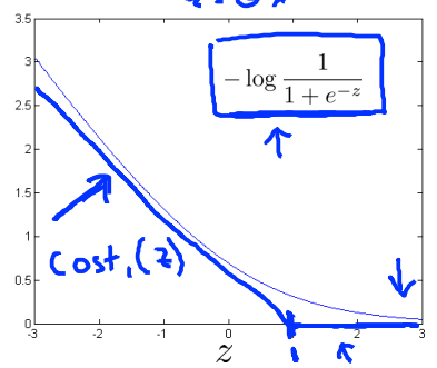 - $y=0$일 때 얻어지는 $L=-\log(1-h_\theta(x))$ 를 $cost_0(z)$로 바꾼다 ($z=\theta^Tx$). -  - 결과적으로 regularization term까지 포함한 logistic regression의 cost function (decision boundary)은 다음과 같이 바뀔 수 있다. Logistic regression $\displaystyle\min_{\theta}\frac{1}{m}\left[\sum_{i=1}^{m}y^{(i)}\operatorname{cost}_{1}\left(\theta^{T}x^{(i)}\right)+\left(1-y^{(i)}\right)\operatorname{cost}_{0}\left(\theta^{T}x^{(i)}\right)\right]+\frac{\lambda}{2m}\sum_{j=1}^{n}\theta_{j}^{2}$ - Support Vector Machine $\displaystyle\min_{\theta}C\left[\sum_{i=1}^{m}y^{(i)}\operatorname{cost}_{1}\left(\theta^{T}x^{(i)}\right)+\left(1-y^{(i)}\right)\operatorname{cost}_{0}\left(\theta^{T}x^{(i)}\right)\right]+\frac{1}{2}\sum_{j=1}^{n}\theta_{j}^{2}$ - 여기서 $C=\frac{1}{\lambda}$일 경우 Logistic Regression의 식과 동일한 최적화 $\theta$값을 가질 것이다. - Decision Boundary - Logistic regression과 마찬가지로, SVM도 $y^{(i)}=1$일 경우와 $y^{(i)}=0$일 경우로 나눠볼 수 있다. - SVM의 decision boundary의 두 가지 case - $y^{(i)}=1$ 의 경우는 $\theta^Tx^{(i)}\ge1$ 를 만족해야 한다 ($cost_1(z)$ 그림 참조). - $y^{(i)}=0$ 의 경우는 $\theta^Tx^{(i)}\le-1$ 를 만족해야 한다 ($cost_0(z)$ 그림 참조). - 각각의 경우를 고려하면, ($cost_1(z)$ 또는 $cost_0(z)$가 0이 되므로), SVM은 아래와 같이 심플하게 표현된다 : $\displaystyle\min_{\theta}C*0+\frac{1}{2}\sum_{j=1}^{n}\theta_{j}^{2}=\min_{\theta}\sum_{j=1}^{n}\theta_{j}^{2}$ - 즉, SVM Decision Boundary는 $\theta$라는 vector와 $x^{(i)}$라는 벡터의 [[dot product]]이라고 생각할 수 있다. - 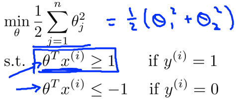 - $\theta^Tx^{(i)}=p^{(i)}\cdot||\theta||=\theta_1x^{(i)}_1+\theta_2x^{(i)}_2$ 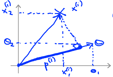 ## B.1) Large Margin Intuition - SVM은 분류된 점에 대해서 가장 가까운 학습 데이터와 가장 먼 거리를 가지는 boundary를 찾는다. - 만약, 그러지 못한(먼 거리를 가지지 못한) boundary를 가진다면, 어떻게 되는가? - 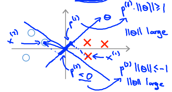 - 위의 그림에서 O와 X는 boundary에 상당히 가깝다. - boundary와 수직인 $\theta$와 각 data들 $x^{(i)}$의 내적을 고려할 경우 $p^{(i)}$ 값은 상당히 작으므로, 올바른 분류를 위해서는 $\|\theta\|$가 커야한다. - 올바른 분류란, O와 X를 위해 $p^{(i)}\cdot\|\theta\|\ge1$ 또는 $p^{(i)}\cdot\|\theta\|\le-1$를 만족해야 하는 것을 의미한다. - 그런데, $\|\theta\|$가 커지면, cost function이 커지므로, 이를 최소화 하는 방향으로 boundary를 조정하게 된다. - 최적의 boundary는 아래와 같이 만들어 진다. - 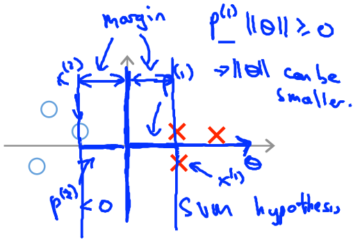 - 위 그림에서 O와 X는 boundary에 충분히 멀다. - boundary와 수직인 $\theta$와 각 data들 $x^{(i)}$의 내적을 고려할 경우 $p^{(i)}$ 값은 상당히 크므로, 올바른 분류를 위해서는 $\|\theta\|$가 작아야한다. - $\|\theta\|$가 작아지면, cost function도 작아지므로, SVM이 올바르게 학습되는 것을 확인할 수 있다. - ## Kernels - 추가적인 features들을 활용해서 complex non-linear boundary를 구성할 수 있게 도와주는 function - - Gaussian Kernel - - $exp(−2*σ*2∥*x*1−*l*(1)∥)$