Megatron-DeepSpeed 의 3D 병렬 처리
Megatron-DeepSpeed 는 대규모 모델을 효율적으로 학습시키기 위해 3D 병렬 처리 방식을 구현합니다. 여기서는 이 3D 병렬 처리의 주요 구성 요소들을 간단히 설명하겠습니다.
A.1) DataParallel (DP)
DataParallel 은 동일한 모델 설정을 여러 번 복제하고, 각 복제본에 데이터의 일부를 할당하여 병렬로 처리하는 방식입니다. 모든 복제본은 각 학습 단계가 끝날 때 동기화됩니다. 즉, 여러 GPU 에서 같은 모델을 사용해 서로 다른 데이터를 동시에 처리하고, 그 결과를 마지막에 합치는 방식입니다.
A.2) TensorParallel (TP)
TensorParallel 은 텐서를 여러 조각으로 나누어 각각의 조각이 지정된 GPU 에 할당되는 방식입니다. 각 텐서 조각은 별도로 병렬로 처리되며, 학습 단계가 끝나면 결과가 동기화됩니다. 이는 텐서를 가로 방향으로 나누어 작업하는 “수평적 병렬화”라고 볼 수 있습니다.
A.3) PipelineParallel (PP)
PipelineParallel 은 모델을 층 단위로 나누어 각 층 또는 몇 개의 층이 하나의 GPU 에 할당되는 방식입니다. 즉, 모델이 수직적으로 분할되어 각 GPU 는 파이프라인의 다른 단계를 동시에 처리하며, 배치 (batch) 의 작은 부분을 작업합니다.
A.4) Zero Redundancy Optimizer (ZeRO)
ZeRO 는 TensorParallel 과 유사하게 텐서를 샤딩 (sharding) 하지만, 차이점은 순방향 (forward) 또는 역방향 (backward) 계산 시 전체 텐서가 재구성된다는 점입니다. 따라서 모델 구조를 변경할 필요 없이 사용할 수 있습니다. 또한 제한된 GPU 메모리를 보완하기 위한 다양한 오프로드 (offloading) 기술도 지원합니다.
B) Data Parallelism
C) 병렬 처리
대부분의 소수 GPU 를 사용하는 사용자들은 DistributedDataParallel(DDP) 방식에 익숙할 것입니다. 이 방법은 모델을 각 GPU 에 완전히 복제한 후, 매 반복 (iteration) 마다 모든 모델이 서로 상태를 동기화하는 방식입니다. 이를 통해 학습 속도를 높일 수 있지만, 이 방법은 모델이 단일 GPU 에 적합할 때만 효과적입니다.
C.1) ZeRO Data Parallelism
ZeRO-powered data parallelism (ZeRO-DP) is described on the following diagram from this blog post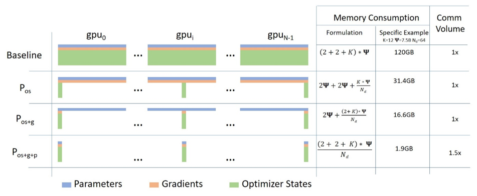
병렬 처리는 처음에는 복잡하게 느껴질 수 있지만, 실제로는 간단한 개념입니다. 기본적으로 DDP(Distributed Data Parallel) 와 비슷하지만, 전체 모델의 파라미터나 그래디언트, 옵티마이저 상태를 모든 GPU 에 복제하는 대신, 각 GPU 가 그 중 일부만 저장합니다.
그리고 실행 시 특정 레이어의 전체 파라미터가 필요할 때는 모든 GPU 가 서로 부족한 부분을 동기화하여 공유합니다. 이 방식이 바로 병렬 처리의 핵심입니다.
이 기능은 DeepSpeed 에서 구현되었습니다.
D) Tensor Parallelism
In Tensor Parallelism (TP) each GPU processes only a slice of a tensor and only aggregates the full tensor for operations that require the whole thing.
In this section we use concepts and diagrams from the Megatron-LM paper: Efficient Large-Scale Language Model Training on GPU Clusters.
The main building block of any transformer is a fully connected nn.Linear followed by a nonlinear activation GeLU.
Following the Megatron paper’s notation, we can write the dot-product part of it as Y = GeLU(XA), where X and Y are the input and output vectors, and A is the weight matrix.
If we look at the computation in matrix form, it’s easy to see how the matrix multiplication can be split between multiple GPUs: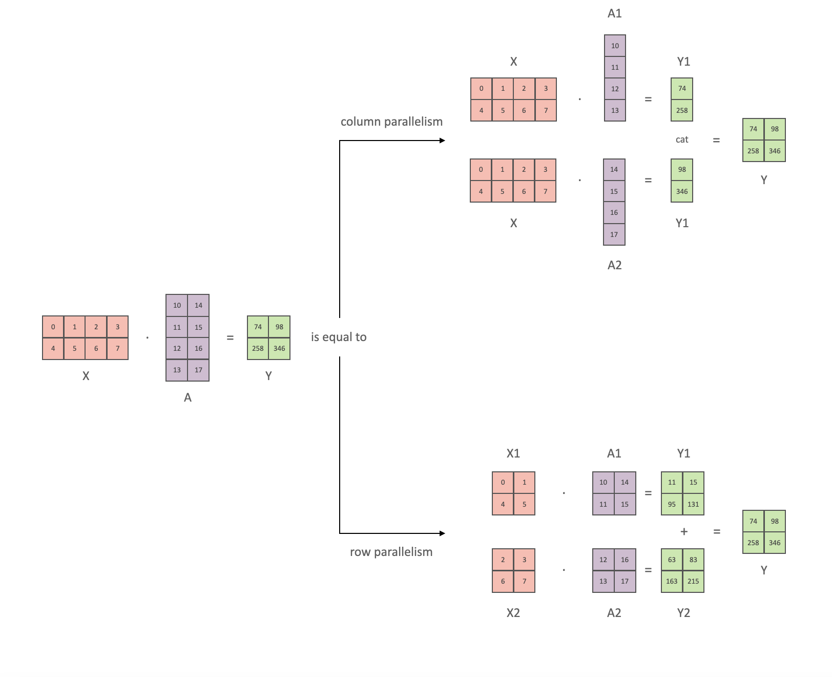
If we split the weight matrix A column-wise across N GPUs and perform matrix multiplications XA_1 through XA_n in parallel, then we will end up with N output vectors Y_1, Y_2, …, Y_n which can be fed into GeLU independently: . Notice with the Y matrix split along the columns, we can split the second GEMM along its rows so that it takes the output of the GeLU directly without any extra communication.
Using this principle, we can update an MLP of arbitrary depth, while synchronizing the GPUs after each row-column sequence. The Megatron-LM paper authors provide a helpful illustration for that: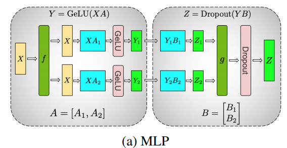
Here f is an identity operator in the forward pass and all reduce in the backward pass while g is an all reduce in the forward pass and identity in the backward pass.
Parallelizing the multi-headed attention layers is even simpler, since they are already inherently parallel, due to having multiple independent heads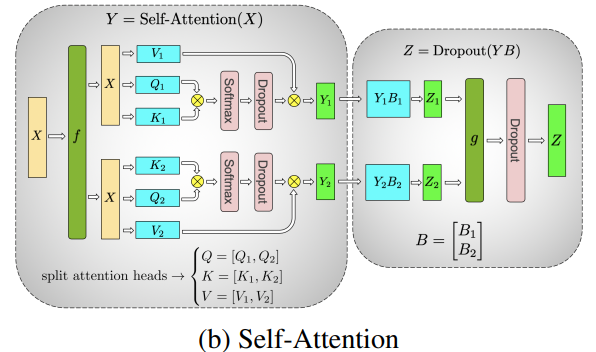
Special considerations: Due to the two all reduces per layer in both the forward and backward passes, TP requires a very fast interconnect between devices. Therefore it’s not advisable to do TP across more than one node, unless you have a very fast network. In our case the inter-node was much slower than PCIe. Practically, if a node has 4 GPUs, the highest TP degree is therefore 4. If you need a TP degree of 8, you need to use nodes that have at least 8 GPUs.
This component is implemented by Megatron-LM. Megatron-LM has recently expanded tensor parallelism to include sequence parallelism that splits the operations that cannot be split as above, such as LayerNorm, along the sequence dimension. The paper Reducing Activation Recomputation in Large Transformer Models provides details for this technique. Sequence parallelism was developed after BLOOM was trained so not used in the BLOOM training.
E) 파이프라인 병렬 처리 (Pipeline Parallelism)
Naive Pipeline Parallelism(naive PP) 은 모델의 여러 층을 여러 GPU 에 분산시키고, 데이터를 각 GPU 로 순차적으로 이동시키는 방식입니다. 마치 하나의 큰 GPU 처럼 작동하는 것처럼 보이죠. 이 메커니즘은 비교적 간단합니다. 원하는 층을 .to() 명령어를 사용해 특정 장치로 전환하면, 데이터가 해당 층을 통과할 때마다 자동으로 그 장치로 이동하게 됩니다. 나머지 부분은 수정하지 않아도 됩니다.
이 방식은 수직적인 모델 병렬 처리를 수행합니다. 대부분의 모델이 그려지는 방식을 떠올리면, 우리는 층을 수직으로 나누게 됩니다. 예를 들어, 아래와 같은 8 층짜리 모델을 생각해볼 수 있습니다:
===================  ===================
|  0 | 1 | 2 | 3  |  |  4 | 5 | 6 | 7  |
===================  ===================
        GPU0                 GPU1
we just sliced it in 2 vertically, placing layers 0-3 onto GPU0 and 4-7 to GPU1.
Now while data travels from layer 0 to 1, 1 to 2 and 2 to 3 this is just like the forward pass of a normal model on a single GPU. But when data needs to pass from layer 3 to layer 4 it needs to travel from GPU0 to GPU1 which introduces a communication overhead. If the participating GPUs are on the same compute node (e.g. same physical machine) this copying is pretty fast, but if the GPUs are located on different compute nodes (e.g. multiple machines) the communication overhead could be significantly larger.
Then layers 4 to 5 to 6 to 7 are as a normal model would have and when the 7th layer completes we often need to send the data back to layer 0 where the labels are (or alternatively send the labels to the last layer). Now the loss can be computed and the optimizer can do its work.
Problems:
- the main deficiency and why this one is called “naive” PP, is that all but one GPU is idle at any given moment. So if 4 GPUs are used, it’s almost identical to quadrupling the amount of memory of a single GPU, and ignoring the rest of the hardware. Plus there is the overhead of copying the data between devices. So 4x 6GB cards will be able to accommodate the same size as 1x 24GB card using naive PP, except the latter will complete the training faster, since it doesn’t have the data copying overhead. But, say, if you have 40GB cards and need to fit a 45GB model you can with 4x 40GB cards (but barely because of the gradient and optimizer states).
- shared embeddings may need to get copied back and forth between GPUs.
Pipeline Parallelism (PP) is almost identical to a naive PP described above, but it solves the GPU idling problem, by chunking the incoming batch into micro-batches and artificially creating a pipeline, which allows different GPUs to concurrently participate in the computation process.
The following illustration from the GPipe paper shows the naive PP on the top, and PP on the bottom:
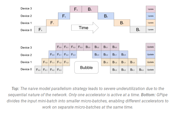
It’s easy to see from the bottom diagram how PP has fewer dead zones, where GPUs are idle. The idle parts are referred to as the “bubble”.
Both parts of the diagram show parallelism that is of degree 4. That is 4 GPUs are participating in the pipeline. So there is the forward path of 4 pipe stages F0, F1, F2 and F3 and then the return reverse order backward path of B3, B2, B1 and B0.
PP introduces a new hyper-parameter to tune that is called chunks. It defines how many chunks of data are sent in a sequence through the same pipe stage. For example, in the bottom diagram, you can see that chunks=4. GPU0 performs the same forward path on chunk 0, 1, 2 and 3 (F0,0, F0,1, F0,2, F0,3) and then it waits for other GPUs to do their work and only when their work is starting to be complete, does GPU0 start to work again doing the backward path for chunks 3, 2, 1 and 0 (B0,3, B0,2, B0,1, B0,0).
Note that conceptually this is the same concept as gradient accumulation steps (GAS). PyTorch uses chunks, whereas DeepSpeed refers to the same hyper-parameter as GAS.
Because of the chunks, PP introduces the concept of micro-batches (MBS). DP splits the global data batch size into mini-batches, so if you have a DP degree of 4, a global batch size of 1024 gets split up into 4 mini-batches of 256 each (1024/4). And if the number of chunks (or GAS) is 32 we end up with a micro-batch size of 8 (256/32). Each Pipeline stage works with a single micro-batch at a time.
To calculate the global batch size of the DP + PP setup we then do: mbs*chunks*dp_degree (8*32*4=1024).
Let’s go back to the diagram.
With chunks=1 you end up with the naive PP, which is very inefficient. With a very large chunks value you end up with tiny micro-batch sizes which could be not very efficient either. So one has to experiment to find the value that leads to the highest efficient utilization of the GPUs.
While the diagram shows that there is a bubble of “dead” time that can’t be parallelized because the last forward stage has to wait for backward to complete the pipeline, the purpose of finding the best value for chunks is to enable a high concurrent GPU utilization across all participating GPUs which translates to minimizing the size of the bubble.
This scheduling mechanism is known as all forward all backward. Some other alternatives are one forward one backward and interleaved one forward one backward.
While both Megatron-LM and DeepSpeed have their own implementation of the PP protocol, Megatron-DeepSpeed uses the DeepSpeed implementation as it’s integrated with other aspects of DeepSpeed.
One other important issue here is the size of the word embedding matrix. While normally a word embedding matrix consumes less memory than the transformer block, in our case with a huge 250k vocabulary, the embedding layer needed 7.2GB in bf16 weights and the transformer block is just 4.9GB. Therefore, we had to instruct Megatron-Deepspeed to consider the embedding layer as a transformer block. So we had a pipeline of 72 layers, 2 of which were dedicated to the embedding (first and last). This allowed to balance out the GPU memory consumption. If we didn’t do it, we would have had the first and the last stages consume most of the GPU memory, and 95% of GPUs would be using much less memory and thus the training would be far from being efficient.
F) DP+PP
The following diagram from the DeepSpeed pipeline tutorial demonstrates how one combines DP with PP.
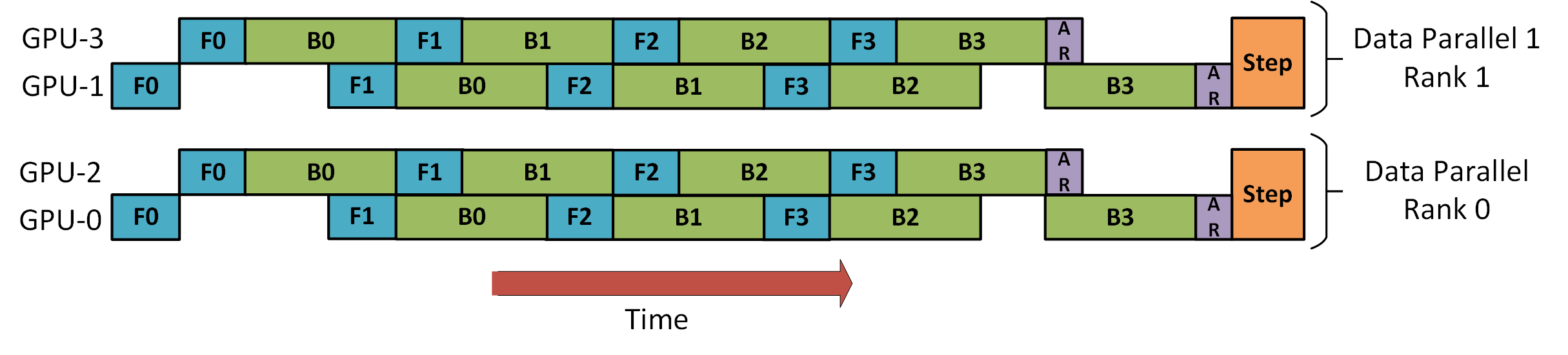
Here it’s important to see how DP rank 0 doesn’t see GPU2 and DP rank 1 doesn’t see GPU3. To DP there are just GPUs 0 and 1 where it feeds data as if there were just 2 GPUs. GPU0 “secretly” offloads some of its load to GPU2 using PP. And GPU1 does the same by enlisting GPU3 to its aid.
Since each dimension requires at least 2 GPUs, here you’d need at least 4 GPUs.
G) DP+PP+TP
To get an even more efficient training PP is combined with TP and DP which is called 3D parallelism. This can be seen in the following diagram.
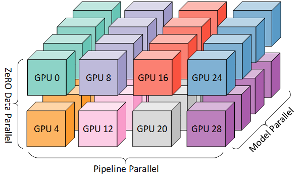
This diagram is from a blog post 3D parallelism: Scaling to trillion-parameter models, which is a good read as well.
Since each dimension requires at least 2 GPUs, here you’d need at least 8 GPUs for full 3D parallelism.
H) ZeRO DP+PP+TP
One of the main features of DeepSpeed is ZeRO, which is a super-scalable extension of DP. It has already been discussed in ZeRO Data Parallelism. Normally it’s a standalone feature that doesn’t require PP or TP. But it can be combined with PP and TP.
When ZeRO-DP is combined with PP (and optionally TP) it typically enables only ZeRO stage 1, which shards only optimizer states. ZeRO stage 2 additionally shards gradients, and stage 3 also shards the model weights.
While it’s theoretically possible to use ZeRO stage 2 with Pipeline Parallelism, it will have bad performance impacts. There would need to be an additional reduce-scatter collective for every micro-batch to aggregate the gradients before sharding, which adds a potentially significant communication overhead. By nature of Pipeline Parallelism, small micro-batches are used and instead the focus is on trying to balance arithmetic intensity (micro-batch size) with minimizing the Pipeline bubble (number of micro-batches). Therefore those communication costs are going to hurt.
In addition, there are already fewer layers than normal due to PP and so the memory savings won’t be huge. PP already reduces gradient size by 1/PP, and so gradient sharding savings on top of that are less significant than pure DP.
ZeRO stage 3 can also be used to train models at this scale, however, it requires more communication than the DeepSpeed 3D parallel implementation. After careful evaluation in our environment which happened a year ago we found Megatron-DeepSpeed 3D parallelism performed best. Since then ZeRO stage 3 performance has dramatically improved and if we were to evaluate it today perhaps we would have chosen stage 3 instead.
I) BF16Optimizer
Training huge LLM models in FP16 is a no-no.
We have proved it to ourselves by spending several months training a 104B model which as you can tell from the tensorboard was but a complete failure. We learned a lot of things while fighting the ever diverging lm-loss:
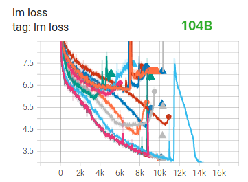
and we also got the same advice from the Megatron-LM and DeepSpeed teams after they trained the 530B model. The recent release of OPT-175B too reported that they had a very difficult time training in FP16.
So back in January as we knew we would be training on A100s which support the BF16 format Olatunji Ruwase developed a BF16Optimizer which we used to train BLOOM.
If you are not familiar with this data format, please have a look at the bits layout. The key to BF16 format is that it has the same exponent as FP32 and thus doesn’t suffer from overflow FP16 suffers from a lot! With FP16, which has a max numerical range of 64k, you can only multiply small numbers. e.g. you can do 250*250=62500, but if you were to try 255*255=65025 you got yourself an overflow, which is what causes the main problems during training. This means your weights have to remain tiny. A technique called loss scaling can help with this problem, but the limited range of FP16 is still an issue when models become very large.
BF16 has no such problem, you can easily do 10_000*10_000=100_000_000 and it’s no problem.
Of course, since BF16 and FP16 have the same size of 2 bytes, one doesn’t get a free lunch and one pays with really bad precision when using BF16. However, if you remember the training using stochastic gradient descent and its variations is a sort of stumbling walk, so if you don’t get the perfect direction immediately it’s no problem, you will correct yourself in the next steps.
Regardless of whether one uses BF16 or FP16 there is also a copy of weights which is always in FP32 - this is what gets updated by the optimizer. So the 16-bit formats are only used for the computation, the optimizer updates the FP32 weights with full precision and then casts them into the 16-bit format for the next iteration.
All PyTorch components have been updated to ensure that they perform any accumulation in FP32, so no loss happening there.
One crucial issue is gradient accumulation, and it’s one of the main features of pipeline parallelism as the gradients from each microbatch processing get accumulated. It’s crucial to implement gradient accumulation in FP32 to keep the training precise, and this is what BF16Optimizer does.
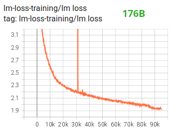
Besides other improvements we believe that using BF16 mixed precision training turned a potential nightmare into a relatively smooth process which can be observed from the following lm loss graph:
J) Fused CUDA Kernels
The GPU performs two things. It can copy data to/from memory and perform computations on that data. While the GPU is busy copying the GPU’s computations units idle. If we want to efficiently utilize the GPU we want to minimize the idle time.
A kernel is a set of instructions that implements a specific PyTorch operation. For example, when you call torch.add, it goes through a PyTorch dispatcher which looks at the input tensor(s) and various other things and decides which code it should run, and then runs it. A CUDA kernel is a specific implementation that uses the CUDA API library and can only run on NVIDIA GPUs.
Now, when instructing the GPU to compute c = torch.add(a, b); e = torch.max([c,d]), a naive approach, and what PyTorch will do unless instructed otherwise, is to launch two separate kernels, one to perform the addition of a and b and another to find the maximum value between c and d. In this case, the GPU fetches from its memory a and b, performs the addition, and then copies the result back into the memory. It then fetches c and d and performs the max operation and again copies the result back into the memory.
If we were to fuse these two operations, i.e. put them into a single “fused kernel”, and just launch that one kernel we won’t copy the intermediary result c to the memory, but leave it in the GPU registers and only need to fetch d to complete the last computation. This saves a lot of overhead and prevents GPU idling and makes the whole operation much more efficient.
Fused kernels are just that. Primarily they replace multiple discrete computations and data movements to/from memory into fused computations that have very few memory movements. Additionally, some fused kernels rewrite the math so that certain groups of computations can be performed faster.
To train BLOOM fast and efficiently it was necessary to use several custom fused CUDA kernels provided by Megatron-LM. In particular there is an optimized kernel to perform LayerNorm as well as kernels to fuse various combinations of the scaling, masking, and softmax operations. The addition of a bias term is also fused with the GeLU operation using PyTorch’s JIT functionality. These operations are all memory bound, so it is important to fuse them to maximize the amount of computation done once a value has been retrieved from memory. So, for example, adding the bias term while already doing the memory bound GeLU operation adds no additional time. These kernels are all available in the Megatron-LM repository.
K) Datasets
Another important feature from Megatron-LM is the efficient data loader. During start up of the initial training each data set is split into samples of the requested sequence length (2048 for BLOOM) and index is created to number each sample. Based on the training parameters the number of epochs for a dataset is calculated and an ordering for that many epochs is created and then shuffled. For example, if a dataset has 10 samples and should be gone through twice, the system first lays out the samples indices in order [0, …, 9, 0, …, 9] and then shuffles that order to create the final global order for the dataset. Notice that this means that training will not simply go through the entire dataset and then repeat, it is possible to see the same sample twice before seeing another sample at all, but at the end of training the model will have seen each sample twice. This helps ensure a smooth training curve through the entire training process. These indices, including the offsets into the base dataset of each sample, are saved to a file to avoid recomputing them each time a training process is started. Several of these datasets can then be blended with varying weights into the final data seen by the training process.
L) Embedding LayerNorm
While we were fighting with trying to stop 104B from diverging we discovered that adding an additional LayerNorm right after the first word embedding made the training much more stable.
This insight came from experimenting with bitsandbytes which contains a StableEmbedding which is a normal Embedding with layernorm and it uses a uniform xavier initialization.
M) Positional Encoding
We also replaced the usual positional embedding with an AliBi - based on the paper: Train Short, Test Long: Attention with Linear Biases Enables Input Length Extrapolation, which allows to extrapolate for longer input sequences than the ones the model was trained on. So even though we train on sequences with length 2048 the model can also deal with much longer sequences during inference.
N) Training Difficulties
With the architecture, hardware and software in place we were able to start training in early March 2022. However, it was not just smooth sailing from there. In this section we discuss some of the main hurdles we encountered.
There were a lot of issues to figure out before the training started. In particular we found several issues that manifested themselves only once we started training on 48 nodes, and won’t appear at small scale. E.g., CUDA_LAUNCH_BLOCKING=1 was needed to prevent the framework from hanging, and we needed to split the optimizer groups into smaller groups, otherwise the framework would again hang. You can read about those in detail in the training prequel chronicles.
The main type of issue encountered during training were hardware failures. As this was a new cluster with about 400 GPUs, on average we were getting 1-2 GPU failures a week. We were saving a checkpoint every 3h (100 iterations) so on average we would lose 1.5h of training on hardware crash. The Jean Zay sysadmins would then replace the faulty GPUs and bring the node back up. Meanwhile we had backup nodes to use instead.
We have run into a variety of other problems that led to 5-10h downtime several times, some related to a deadlock bug in PyTorch, others due to running out of disk space. If you are curious about specific details please see training chronicles.
We were planning for all these downtimes when deciding on the feasibility of training this model - we chose the size of the model to match that feasibility and the amount of data we wanted the model to consume. With all the downtimes we managed to finish the training in our estimated time. As mentioned earlier it took about 1M compute hours to complete.
One other issue was that SLURM wasn’t designed to be used by a team of people. A SLURM job is owned by a single user and if they aren’t around, the other members of the group can’t do anything to the running job. We developed a kill-switch workaround that allowed other users in the group to kill the current process without requiring the user who started the process to be present. This worked well in 90% of the issues. If SLURM designers read this - please add a concept of Unix groups, so that a SLURM job can be owned by a group.
As the training was happening 24/7 we needed someone to be on call - but since we had people both in Europe and West Coast Canada overall there was no need for someone to carry a pager, we would just overlap nicely. Of course, someone had to watch the training on the weekends as well. We automated most things, including recovery from hardware crashes, but sometimes a human intervention was needed as well.
O) Conclusion
The most difficult and intense part of the training was the 2 months leading to the start of the training. We were under a lot of pressure to start training ASAP, since the resources allocation was limited in time and we didn’t have access to A100s until the very last moment. So it was a very difficult time, considering that the BF16Optimizer was written in the last moment and we needed to debug it and fix various bugs. And as explained in the previous section we discovered new problems that manifested themselves only once we started training on 48 nodes, and won’t appear at small scale.
But once we sorted those out, the training itself was surprisingly smooth and without major problems. Most of the time we had one person monitoring the training and only a few times several people were involved to troubleshoot. We enjoyed great support from Jean Zay’s administration who quickly addressed most needs that emerged during the training.
Overall it was a super-intense but very rewarding experience.
Training large language models is still a challenging task, but we hope by building and sharing this technology in the open others can build on top of our experience.